
For any "Introduction to Machine Learning" classes, two questions get asked a lot of times and that is “What is gradient descent?” and “How does gradient descent figure in Machine Learning?”.
Through the years of training I have given, I have "sharpened" an explanation on what gradient descent is and why is it the “essential ingredient” in most machine learning models.
Note: To understand the explanation, the assumption is the reader understands Calculus, especially Differentiation up to an order of 2.
Cost Function
For those learning or has learnt about Machine Learning, you know that each Machine Learning model has a cost function. To explain it very briefly, it is a way to determine how well the machine learning model has performed given the different values of each parameters/coefficients.
For example, the linear regression model, the parameters will be the two coefficients, Beta 1 and Beta 2.
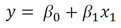
The cost function will be the sum of least square methods.
Since the cost function is a function of the parameters Beta 1 and Beta 2, we can plot out the cost function with each value of Beta. (i.e. Given the value of each coefficient, we can refer to the cost function to know how well the machine learning model has performed. )
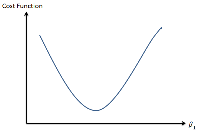
Given that there are many parameters, you can imagine that once the cost function is determined, the contours of a multi-dimension plane is laid out. (similar to a mountainous region in a 3 dimensions).
NOTE: This is where there is a lot of confusion. Basically, I have seen many people got confused by the horizontal axis. They thought that the horizontal axis is actually Xs, or the independent variables which is not true because the Xs will remain the same throughout the training phase. Always remember during the training phase, we are focused on selecting the ‘best’ value for the parameters (i.e. the coefficients, the Betas).
When we are training the model, we are trying to the find the values of the coefficients (the Betas, for the case of linear regression) that will give us the lowest cost. In other words, for the case of linear regression, we are finding the value of the coefficients that will reduce the cost to the minimum a.k.a the lowest point in the mountainous region.
“Gradient” Descent
Let us look into the training phase of the model now.
So now imagine we put an agent into this multi-dimension plane (remember the mountainous region), the starting position is randomly given (i.e. randomly assigned a value for each coefficient). This randomly assigned starting position is known as “Initialization” in the machine learning world, and it is a whole research area altogether.
This agent can only see one thing and that is the gradient at the point where it is standing, a.k.a rate of change of cost given a unit change in coefficient. This intuition of the gradient is gotten from the first order differentiation in Calculus. That explains the “Gradient” of the Gradient Descent.
Gradient “Descent”
If you studied any materials on gradient descent, you will come across another technical term known as the Learning Rate. The learning rate actually refers to how large a step the agent takes when traveling in the “mountainous region”, meaning how large a change in the parameters (again a reminder, its the Beta in this explanation) we are taking. So if the gradient is steep at the standing point and you take a large step, you will see a large decrease in the cost.
Alternatively, if the gradient is small (gradient is close to zero), then even if a large step is taken, given that the gradient is small, the change in the cost will be small as well.
Putting It All Together
Thus in gradient descent, at each point the agent is in, the agent only knows the GRADIENT (for each parameter) and the width of the STEP to take. With the gradient and the step taken into account, the current value of each parameters will be updated. With the new values of the parameters, the gradients are re-calculated again and together with the step, the new value of the parameters is updated. This keeps on repeating until we get to convergence (which we will discuss in a while). Given many repeated steps, the agent will slowly DESCENT to the lowest point in the mountainous region.
Now you may ask why the agent will move to the lowest point and not do an ascent. That I will leave it to the readers to find out more but let me provide some direction for research. It has something to do with the fact that cost functions are convex function and how the value of the parameters are updated.
Convergence
Once the agent, after many steps, realize the cost does not decrease much and it is stuck very near a particular point (minima), technically this is known as convergence. The value of the parameters at that very last step is known as the ‘best’ set of parameters (in the case of the linear regression model, we have the ‘best’ value for both Betas). And we have a trained model.
In conclusion, gradient descent is a way for us to calculate the best set of values for the parameters of concern.
The steps are as follows:
1 — Given the gradient, calculate the change in parameter with respect to the size of step taken.
2 — With the new value of parameter, calculate the new gradient.
3 — Go back to step 1.
And the sequence of steps will stop once we hit convergence. I hope this helps with your understanding of gradient descent.
So let me welcome you to the world of gradient descent and if you are adventurous enough (which I hope you do after the blog post), do check out this blog post by Sebastian Ruder that talks about other variants of gradient descent algorithms.
I hope this blog post has been useful. Have fun in your Data Science learning journey and do visit my other blog posts. Keep in touch on LinkedIn or Twitter, else subscribe to my newsletter to find out what I am thinking, doing or learning. :)